DIY Haar wavelet transform

This post walks through an implementation of the Haar wavelet transform.

Background

Why do we care about wavelet transforms? At a high level, wavelet transforms allow you to analyze the frequency content of your data while achieving different temporal (or spatial) resolutions for different frequencies. They’re useful in a variety of applications including JPEG 2000 compression.

According to the uncertainty principle for signal processing, there is a trade-off between temporal/spatial resolution and frequency resolution. As we’ll see later in this post, our wavelet transformed image will have low spatial resolution with high frequency resolution for lower frequencies but high spatial resolution with low frequency resolution for higher frequencies. A Fourier transform, in contrast, would produce medium spatial resolution with medium frequency resolution for all frequencies.

With that background in place, we’ll demonstrate these concepts with an implementation of the Haar wavelet transform.

Basic Implementation

For our wavelet implementation, an image will be iteratively decomposed into low and high frequency components. The low and high frequency components are created such that the original image can be reconstructed without any loss of information. The low frequency component we’ll refer to as the sum component ($s_{r,c}$) and the high frequency component we’ll refer to as difference ($d_{r,c}$).

$$s_{r,c} = x_{r,2c} + x_{r,2c+1}$$ $$d_{r,c} = x_{r,2c} - x_{r,2c+1}$$

where $x_{5,3}$ would be the pixel value at the $5^{th}$ row and $3^{rd}$ column of the original image.

This can be represented with the following Python code:

evens = x[:, 0::2]
odds = x[:, 1::2]
s = evens + odds
d = evens - odds

Reversing this transform is relatively easy:

$$x_{r,2c} = \frac {s_{r,c} + d_{r,c}} 2$$ $$x_{r,2c+1} = \frac {s_{r,c} - d_{r,c}} 2$$

Similarly, the Python code looks like this:

x[:, 0::2] = (s + d) // 2
x[:, 1::2] = (s - d) // 2

Now let’s apply this transform a single time to the following image:

The transformed image (after converting the image to grayscale) looks like this:

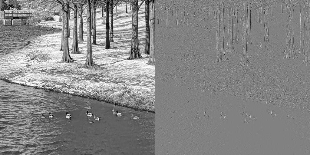
As is usually done for images, we can also perform the same transform across rows instead of columns. I.e.

$$s_{r,c} = x_{2r,c} + x_{2r+1,c}$$ $$d_{r,c} = x_{2r,c} - x_{2r+1,c}$$

Which gives us this:

Typically, the low frequency component in the upper left corner of the image will undergo additional stages of decomposition as shown in the next section.

Iterative Implementation

With the computational pieces just discussed, we can put together the following class which decomposes images into an arbitrary number of levels as we’ll visualize shortly.

class WaveletImage:
    def __init__(self, image: ndarray, axis: int = 1, levels: int = 2) -> None:
        self.axis = axis
        self.lo, self.hi = self.transform(image, self.axis, levels)

    @property
    def pixels(self) -> ndarray:
        lo = norm_image(self.lo if isinstance(self.lo, ndarray) else self.lo.pixels)
        hi = norm_image(self.hi if isinstance(self.hi, ndarray) else self.hi.pixels)
        return np.concatenate([lo, hi], axis=self.axis)

    def inverse_transform(self) -> ndarray:
        lo: ndarray = self.lo if isinstance(self.lo, ndarray) else self.lo.inverse_transform()
        hi: ndarray = self.hi if isinstance(self.hi, ndarray) else self.hi.inverse_transform()
        evens = (lo + hi) // 2
        odds = (lo - hi) // 2
        return interleave(evens, odds, axis=self.axis)

    @staticmethod
    def transform(image: ndarray, axis: int, levels: int) -> Tuple[ndarray, ndarray]:
        if axis == 0:
            evens, odds = image[::2, :], image[1::2, :]
        elif axis == 1:
            evens, odds = image[:, ::2], image[:, 1::2]
        else:
            raise ValueError(f"axis '{axis}' must be 0 or 1")

        lo = WaveletImage(evens + odds, abs(axis - 1), levels - axis) if levels else evens + odds
        hi = WaveletImage(evens - odds, axis=0, levels=0) if axis == 1 else evens - odds

        return lo, hi


def norm_image(x: ndarray) -> ndarray:
    return (x - x.min()) / (x.max() - x.min())


def interleave(a: ndarray, b: ndarray, axis: int) -> ndarray:
    rows, cols = a.shape
    rows, cols = (rows * 2, cols) if axis == 0 else (rows, cols * 2)
    out = np.empty((rows, cols), dtype=a.dtype)
    if axis == 0:
        out[0::2] = a
        out[1::2] = b
    elif axis == 1:
        out[:, 0::2] = a
        out[:, 1::2] = b
    else:
        raise ValueError("interleave only supports axis of 0 or 1")
    return out

If we create a WaveletImage object with levels=1, the result will look like the image we just created in the last section that has both horizontal and vertical decompositions, resulting in 2x2 tiles.

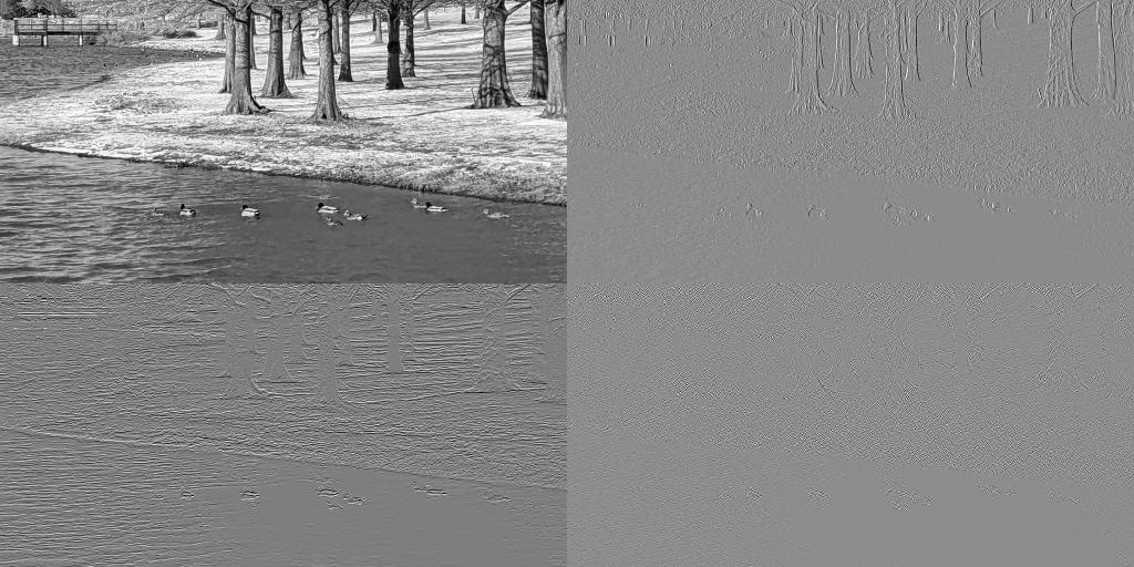
However, things get a bit more interesting when we transform with levels=2. We can see what the result looks like with:

image = WaveletImage(image, levels=2).pixels

plt.imshow(image, cmap="gray")
plt.show()

Which gives us this:

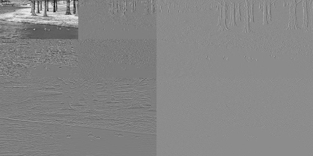
Pretty cool, right? We can add an additional level of decomposition by setting levels=3 as shown below.

image = WaveletImage(image, levels=3).pixels

plt.imshow(image, cmap="gray")
plt.show()

And the result looks like this:

As mentioned at the beginning of this post, low frequency components have higher frequency resolution at the cost of lower spatial resolution while while high frequency components have higher spatial resolution at the cost of lower frequency resolution.

You can see difference in spatial resolution between low and high frequency components by comparing the low frequency component in the upper left hand corner which is at $\frac 1 {64}$ resolution of the original image versus the high frequency component in the lower right hand corner which is at $\frac 1 4$ resolution of the original image.

That’s all for this post! If you have any feedback, please feel free to reach out.

Also, if you enjoyed this post, you may also enjoy my posts LGT wavelet transform from scratch, DIY Metropolis-Hastings and DIY pseudorandom number generator.

Published on 11 March 2022

If you enjoy this blog, please consider supporting me by buying one of my books. 📚
(click here)